This is an Open Access article distributed under the terms of the Creative Commons Attribution Non-Commercial License (http://creativecommons.org/licenses/by-nc/4.0/) which permits unrestricted non-commercial use, distribution, and reproduction in any medium, provided the original work is properly cited.
Systematic reviews and meta-analyses are pivotal for evidence-based decision-making but depend on the availability of precise statistical data. Researchers often encounter studies where essential statistics are missing or presented only in graphs, leading to potential data exclusion and selection bias. This study aims to provide specific methodologies for extracting or reconstructing the statistical parameters required for meta-analysis—specifically effect sizes (MD, OR, RR, HR) and their corresponding variance measures (SD, SE, variance)—from incomplete or graphically reported data. We describe calculation and extraction protocols for five specific scenarios encountered in medical literature: (1) continuous data missing standard deviations; (2) categorical data missing standard errors; (3) calculating risk estimates from frequency tables; (4) extracting continuous data presented solely in graphs; and (5) reconstructing hazard ratios from Kaplan-Meier survival curves. Valid meta-analysis requires both an effect size and a measure of variance. When these are not explicitly reported, they can often be derived from other available statistics or digital extraction from figures. While heterogeneity is inherent in meta-analysis, the methodology allows for error adjustment and robust synthesis. Therefore, preventing data loss via these extraction methods is preferable to excluding studies. Maximizing data inclusion enhances the comprehensive value and statistical power of the final analysis.
With the explosive increase in research output on various clinical topics, academic focus has shifted beyond individual study findings toward the systematic integration of vast datasets to derive rational conclusions. Against this backdrop, meta-analysis emerged in the late 1980s as a cornerstone of research synthesis, quantitatively aggregating preceding studies to provide intuitive and consolidated results. Following continuous methodological evolution, meta-analysis has become an essential research tool not only in the social sciences, such as psychology and pedagogy, but also in the medical and health sciences [1]. By ensuring objectivity in literature selection and quantifying individual findings into pooled effect sizes, meta-analysis contributes decisively to decision-making in evidence-based medicine (EBM) [2,3].
Since the Cochrane Collaboration established the methodology for systematic reviews [2], pooled effect sizes in meta-analyses have typically been presented as mean differences (MD), odds ratios (OR), relative risks (RR), or hazard ratios (HR) [4-6]. Conducting such analyses requires the extraction of specific statistical information from individual studies. For instance, when effect sizes are reported as MD or risk ratios (OR, RR, or HR), both the point estimate and its corresponding 95% confidence interval (CI) or standard error (SE) must be retrieved [1]. Similarly, for proportion data expressed as percentages, most meta-analyses require the sample size, effect size, and 95% CI [1,3].
However, researchers often encounter difficulties calculating accurate summary statistics when individual papers fail to explicitly report these values. Excluding such studies can introduce selection bias; therefore, maximizing the utility of available statistical information is crucial. For continuous data, if the standard deviation (SD) is not directly stated, it can be calculated using sample sizes, variances, or SEs [7,8]. If the data remain insufficient for direct derivation, alternative methods, such as imputing the largest SD from other included studies, may be considered [9,10]. In the case of time-to-event data, when statistical information is presented only through graphs, data must be estimated directly from the visual representations. While some studies have reported using grid paper to visually estimate values from Kaplan-Meier survival curves (KMSC) [11], utilizing high-resolution digital tools is preferable for greater accuracy. To this end, methods for extracting survival data using Python-based programs have been developed [12].
Accordingly, this manuscript aims to explore methodologies for back-calculating or extracting the necessary statistical parameters for different data types when primary values are unreported in published literature.
Methods
Missing data can compromise the precision of pooled effect size estimates and introduce bias in meta-analyses. In this study, we operated under the assumption that missing data were missing at random (MAR), implying that the probability of missingness was not dependent on unobserved variables. Furthermore, we calculated estimates assuming that the 95% CIs were symmetrically distributed under a normal distribution.
Fundamentally, meta-analysis synthesizes findings by calculating study-specific weights. This process necessitates the extraction of effect sizes and SEs—or values from which these can be derived, such as variance and 95% CIs—from each individual study. Consequently, obtaining accurate effect sizes and SEs for the intervention in question is a critical priority for researchers.
For Randomized Controlled Trials (RCTs), particularly those conducted since approximately 2007, most studies have been prospectively registered in the web-based database ClinicalTrials.gov to mitigate research misconduct and ensure transparency regarding sponsorship and study background [13]. While not universally mandatory by law, this practice is largely driven by high-impact journals, which typically require a ClinicalTrials.gov registration number as a prerequisite for manuscript submission. Therefore, when including RCTs in a meta-analysis, researchers should prioritize consulting this database to identify potential unpublished but valuable data.
Practical Guidance for Missing Summary Statistics and Extracted Data
Calculation of summary statistics and effect sizes for continuous data
For continuous variables, we calculated the MD, SD, SE, Cohen’s d, and Hedges’ g for both paired groups (e.g., pre- vs. post-intervention; Table 1) and independent groups (Table 2) using the virtual data. While most statistical software automatically computes effect sizes (Cohen’s d and Hedges’ g) upon entry of the sample size, mean, and SD, specific manual adjustments were applied as follows.
In paired group designs (Table 1), in clinical medicine, improvement is typically indicated by a reduction in values (i.e., a negative direction). In this simulation study, change scores were calculated by subtracting baseline values from post-intervention values (Post - Pre), meaning that negative values represent improvement; however, this directionality was adjusted based on the specific research context. Regarding the calculation of the pre-post pooled SD, most individual studies do not report the correlation coefficient (r) between pre- and post-values, consequently, we assumed a conservative correlation coefficient of 0.5 for these calculations, a method explicitly be stated in the meta-analysis methodology [14,15]. Additionally, it is recommended to conduct a sensitivity analysis (Cochrane Handbook for Systematic Reviews of Interventions. Section 6.5.2.8 Imputing standard deviations for changes from baseline) [2].
For independent groups (Treatment vs. Control), we utilized Cohen’s d as the standardized mean difference (SMD). In cases where sample sizes were small, we employed Hedges’ g to correct for small-sample bias (Table 2). When summary statistics were not explicitly reported in individual studies, they were derived using relevant algebraic formulas. For instance, when only the pre- and post-test SDs were available, the pooled SD corresponding to the mean change was calculated (Table 1). Similarly, when the SDs of two independent groups were provided, the pooled SD for the mean difference between the groups was computed (Table 2).
Handling missing standard deviations in continuous data
When SDs were not reported, we derived the SE using the following formulas:
SE=SD/nSE=(CIH-CIL)/(1.96*2)
For continuous outcomes presenting MD as the effect size, we extracted the sample size, mean, and SD. It is crucial to verify whether the extracted values correspond to independent or paired groups before applying the formulas. Generally, the SE is the SD divided by the square root of the sample size. Alternatively, if the 95% CI is provided, the SE can be calculated by subtracting the lower limit (CIL) from the upper limit (CIH) and dividing the result by 3.92.
In instances where these calculations were not feasible, we employed imputation strategies as described in Cochrane Handbook Chapter 6: Choosing effect measures and computing estimates of effect [2].
First, we excluded studies with missing data to calculate a pooled effect size and pooled SD from the remaining studies; this pooled SD was then imputed into the studies with missing values. Alternatively, we imputed the SD from a representative study with high methodological quality (e.g., rigorous design, large sample size) that closely resembled the study with missing data.
Importantly, these handling methods for missing data must be clearly defined in the methodology section. To enhance the robustness of the findings, we recommend conducting a sensitivity analysis comparing results that include imputed data against those that exclude studies with missing values.
Handling missing standard errors in categorical data
For categorical data where the effect size is presented as an OR, RR, or HR, the SE is the square root of the variance (V):
SE=VSE=(log(CIH)-log(CIL))/3.92
Studies often omit the SE and variance but provide the 95% CI. In such cases, the SE can be calculated using the log-transformed CI limits. Log transformation is essential to normalize the data distribution. Furthermore, when conducting meta-analyses on categorical data, effect sizes are log-transformed to calculate the pooled effect size and then back-transformed (exponentiated) to report the final OR, RR, or HR.
Deriving Statistics from Frequency Tables (Categorical Data)
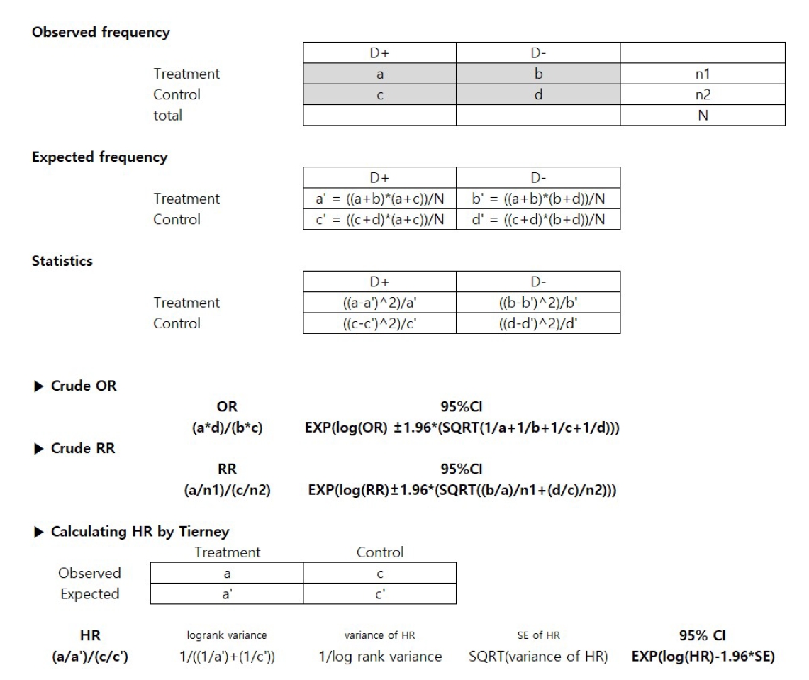
When effect sizes (OR, RR, HR) and related statistics were absent but frequency tables for specific treatments were available, we calculated crude unadjusted risks (Figure 1). OR and RR were calculated using standard statistical formulas, while HRs were estimated using the methodology described by Tierney et al. [16]. We calculated OR and RR based on the observed frequencies in the 2*2 contingency tables. To assess statistical significance, we computed test statistics (e.g., chi-square) by comparing the discrepancy between observed and expected frequencies, providing 95% CIs. In addition, following the method described by Tierney et al. [16], we calculated HR by rearranging the observed and expected frequencies from the patient groups only into the corresponding frequencies for the treatment and control arms.
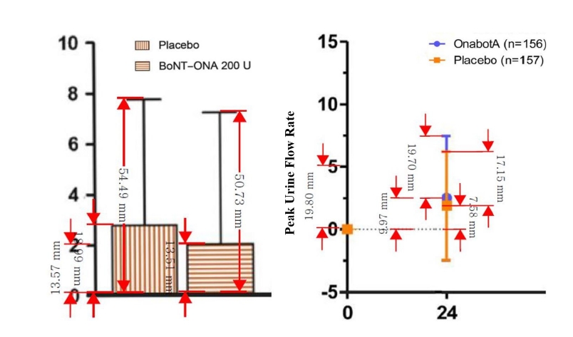
Extracting continuous data from graphical presentations
While the aforementioned methods utilize numerical data, some studies present findings solely through graphs. Given that graphs in modern medical literature are generated by software with standardized axes and ratios, data can be accurately extracted using digital measurement tools such as Adobe Acrobat Reader, WebPlotDigitizer, Plot Digitizer, or Engauge Digitizer [12].
As shown in Figure 2, we extracted mean changes and SDs from bar graphs and box-and-whisker plots using the measurement tool in Adobe Acrobat Reader. By setting a specific segment of the Y-axis as a reference scale, we calculated the values of the target bars or boxes using proportional equations. For example, if a reference measurement of 0 to 5 on the Qmax axis corresponds to 19.80 mm in the software, and the placebo change bar measures 7.58 mm, the actual value is calculated as 1.91 (Calculation: 5 : 19.80 = x : 7.58, therefore x = 1.91).
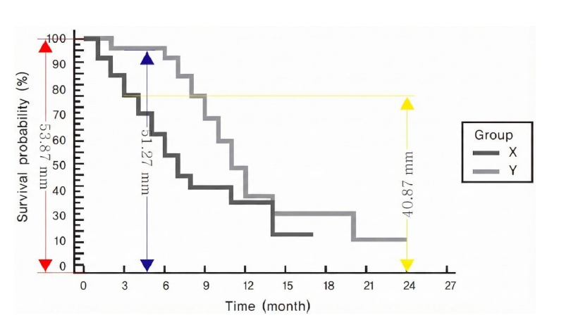
Extracting survival data from graphical presentations
In survival analyses where only Kaplan-Meier survival curves were provided without explicit HRs, we extracted data points from the curves to calculate the HR (Figure 3). The fundamental principle involves determining interval-specific HRs, variance (V), and observed-minus-expected (O-E) events, then synthesizing these to derive a single pooled HR and SE [11,17]. Narrower time intervals typically yield results closer to the raw data.
However, our validity checks revealed significant discrepancies between summary statistics extracted via this method and actual values. This is likely because survival analysis inherently accounts for both time and censoring simultaneously. Inverse calculation from a final static graph cannot fully capture the dynamic censoring information present in the raw data, inevitably leading to deviations from the original effect sizes.
Conclusions
Despite the inherent heterogeneity across individual studies included in a meta-analysis, the methodological framework of this approach allows for the adjustment of various errors, thereby facilitating robust synthesis. Given that the primary objective of meta-analysis is to enable comprehensive decision-making based on a wide array of evidence [1,18-20], it is methodologically preferable to minimize data exclusion due to missing values rather than discarding potentially valuable information. This rigorous approach reflects the rationale behind the PRISMA (Preferred Reporting Items for Systematic Reviews and Meta-Analyses) guidelines, which employ a 27-item checklist to enhance the completeness and establish the transparency of systematic reviews and meta-analyses. [21]
However, this study is subject to certain limitations. We operated under the assumption that the missing data in individual studies were MAR. It is important to acknowledge that the MAR assumption is inherently untestable and cannot be empirically verified. Consequently, to address this uncertainty, we strongly recommend conducting sensitivity analyses that account for reasonable deviations. Comparing results derived from datasets that include imputed missing values against those that exclude them is essential to validate the robustness of the study's conclusions.
Furthermore, excluding studies solely due to missing summary statistics reduces the effective sample size and statistical power, potentially leading to Type II errors where significant effects are overlooked. By employing valid imputation strategies under the MAR assumption, researchers can preserve the integrity of the total sample, ensuring that the synthesized evidence reflects a more complete picture of the available data.
In addition, HRs reconstructed from Kaplan-Meier curves may not fully capture censoring information, potentially leading to discrepancies with the actual HRs. Therefore, this approach should be considered an approximation; priority should be given to obtaining original summary statistics or contacting the study authors whenever possible.
Ultimately, the challenges associated with missing data highlight the critical need for improved reporting standards in primary research. Future clinical trials should strictly adhere to reporting guidelines, such as the CONSORT statement, ensuring that all summary statistics—including means, SD, and CIs—are explicitly reported or archived in public repositories. Such transparency would eliminate the need for post-hoc data extraction or imputation, thereby enhancing the accuracy and reliability of subsequent systematic reviews and meta-analyses.
Notes
Conflict of Interest
The author declares no conflict of interest.
Funding
No funding was received for this work.
Data Availability Statement
Not applicable.
Ethics Approval and Consent to Participate
Not applicable.
Authors Contributions
Jieun Shin and Sung Ryul Shim had full access to all the data in the study and takes responsibility for the integrity of the data and the accuracy of the data analysis. Analysis and interpretation of data: Jieun Shin, Seong-Jang Kim and Sung Ryul Shim. Drafting of the manuscript: Jieun Shin, Taeho Greg Rhee and Sung Ryul Shim. Critical revision of the manuscript for important intellectual content: Jieun Shin, Taeho Greg Rhee and Sung Ryul Shim. Statistical analysis: Jieun Shin and Sung Ryul Shim.
Acknowledgments
None.
Fig. 1.
Calculation of Odds Ratio (OR), Relative Risk (RR), or Hazard Ratio (HR) Using Frequencies
Fig. 2.
Data extraction from graph Using Adobe Acrobat Reader. All values are virtual data. BoNT-ONA, Onabotulinum toxin A; OnabotA, Onabotulinum toxin A
Fig. 3.
Data extraction from Kaplan-Meier survival curve. All values are virtual data
Table 1.
Paired Two Groups (Pre vs. Post)
Treatment
Control
n_pre
m_pre
s_pre
n_post
m_post
s_post
Sdiff
m1
n_pre
m_pre
s_pre
n_post
m_post
s_post
Sdiff
m2
100
20
5
100
10
3
4.359
-10
100
19
4
100
17
3
3.606
-2
m1 = m_post-m_pre
Sdiff = SQRT(s_pre^2+s_post^2-(2*r*s_pre*s_post)) *Since correlation (r) is generally unknown, treat it as 0.5.
n, sample size; m, mean; s, standard deviation; Sdiff, standard deviation of mean difference; m1, mean difference between pre- and post-treatment in the treatment group; m2, mean difference between pre- and post-treatment in the control group.
All values are virtual data.
Table 2.
Independent Two Groups (Treatment vs. Control)
Treatment
Control
MD
Sp
SEmd
Cohen's d
Vd
SEd
J
Hedges' g
Vg
SEg
n1
m1
s1
n2
m2
s2
100
-10
4.359
100
-2
3.606
-8
4.000
0.566
-2.000
0.030
0.173
0.996
-1.992
0.030
0.173
MD = m2-m1
Sp = SQRT(((n1-1)*s1^2+(n2-1)*s2^2)/(n1+n2-2))
SEmd = SQRT(1/n1+1/n2)*Sp
Cohen's d = MD/Sp
Vd = 1/n1+1/n2+Cohen's d^2/(2*(n1+n2))
SEd = SQRT(Vd)
J = (1-(3/(4*(n1+n2)-9)))
Hedges' g = Cohen's d*J
Vg = Vd*J^2
SEg = SQRT(Vg)
n, sample size; m, mean; s, standard deviation; MD, mean difference between treatment and control; Sp, standard deviation of MD (pooling standard deviation); SEmd, standard error of MD; Vd, variance of Cohen’s d; SEd, standard error of Cohen’s d; J, correction factor; Vg, variance of Hedges’ g; SEg, standard error of Hedges’ g.
All values are virtual data.
References
1. Shim SR, Kim SJ. Intervention meta-analysis: application and practice using R software. Epidemiol Health 2019; 41: e2019008.
2. Higgins JPT TJ, Chandler J, Cumpston M, Li T, Page MJ. Cochrane Handbook for Systematic Reviews of Interventions version 6.5 (updated August 2024) [Internet]. The Cochrane Collaboration; 2024 Available from: http://www.cochrane-handbook.org
3. Shim SR. R Meta-Analysis for Medical and Public Health Researchers. 2019.
4. Barratt A, Wyer PC, Hatala R, McGinn T, Dans AL, Keitz S, et al. Tips for learners of evidence-based medicine: 1. Relative risk reduction, absolute risk reduction and number needed to treat. Cmaj 2004; 171: 353-8.
5. Smeeth L, Haines A, Ebrahim S. Numbers needed to treat derived from meta-analyses--sometimes informative, usually misleading. Bmj 1999; 318: 1548-51.
7. Shim SR, Cho YJ, Shin IS, Kim JH. Efficacy and safety of botulinum toxin injection for benign prostatic hyperplasia: a systematic review and meta-analysis. Int Urol Nephrol 2016; 48: 19-30.
8. Shim SR, Kim JH, Choi H, Lee WJ, Kim HJ, Bae MY, et al. General effect of low-dose tamsulosin (0.2 mg) as a first-line treatment for lower urinary tract symptoms associated with benign prostatic hyperplasia: a systematic review and meta-analysis. Curr Med Res Opin 2015; 31: 353-65.
9. Fu R, Vandermeer BW, Shamliyan TA, O’Neil ME, Yazdi F, Fox SH, et al. AHRQ Methods for Effective Health Care Handling Continuous Outcomes in Quantitative Synthesis. Methods Guide for Effectiveness and Comparative Effectiveness Reviews. Rockville (MD), Agency for Healthcare Research and Quality (US). 2008.
10. Idris NRN, Robertson C. The Effects of Imputing the Missing Standard Deviations on the Standard Error of Meta Analysis Estimates. Communications in Statistics - Simulation and Computation 2009; 38: 513-26.
11. Bae JM. A Practical Method for Using a Survival Curve for Meta-analysis. J Health Info Stat 2015; 40: 56-65.
12. Shim S.R, L YH, Hong M.H, Song G.S, Han H.W. Statistical Data Extraction and Validation from Graph for Data Integration and Meta-analysis. The Korea Journal of BigData 2021; 6.
15. Follmann D, Elliott P, Suh I, Cutler J. Variance imputation for overviews of clinical trials with continuous response. J Clin Epidemiol 1992; 45: 769-73.
17. Parmar MK, Torri V, Stewart L. Extracting summary statistics to perform meta-analyses of the published literature for survival endpoints. Stat Med 1998; 17: 2815-34.
21. Page MJ, McKenzie JE, Bossuyt PM, Boutron I, Hoffmann TC, Mulrow CD, et al. The PRISMA 2020 statement: an updated guideline for reporting systematic reviews. BMJ 2021; 372: n71.
Calculating and extracting missing summary statistics for meta-analysis
Fig. 1. Calculation of Odds Ratio (OR), Relative Risk (RR), or Hazard Ratio (HR) Using Frequencies
Fig. 2. Data extraction from graph Using Adobe Acrobat Reader. All values are virtual data. BoNT-ONA, Onabotulinum toxin A; OnabotA, Onabotulinum toxin A
Fig. 3. Data extraction from Kaplan-Meier survival curve. All values are virtual data
Fig. 1.
Fig. 2.
Fig. 3.
Calculating and extracting missing summary statistics for meta-analysis
Treatment
Control
n_pre
m_pre
s_pre
n_post
m_post
s_post
Sdiff
m1
n_pre
m_pre
s_pre
n_post
m_post
s_post
Sdiff
m2
100
20
5
100
10
3
4.359
-10
100
19
4
100
17
3
3.606
-2
Treatment
Control
MD
Sp
SEmd
Cohen's d
Vd
SEd
J
Hedges' g
Vg
SEg
n1
m1
s1
n2
m2
s2
100
-10
4.359
100
-2
3.606
-8
4.000
0.566
-2.000
0.030
0.173
0.996
-1.992
0.030
0.173
Table 1. Paired Two Groups (Pre vs. Post)
m1 = m_post-m_pre
Sdiff = SQRT(s_pre^2+s_post^2-(2*r*s_pre*s_post)) *Since correlation (r) is generally unknown, treat it as 0.5.
n, sample size; m, mean; s, standard deviation; Sdiff, standard deviation of mean difference; m1, mean difference between pre- and post-treatment in the treatment group; m2, mean difference between pre- and post-treatment in the control group.
All values are virtual data.
Table 2. Independent Two Groups (Treatment vs. Control)
MD = m2-m1
Sp = SQRT(((n1-1)*s1^2+(n2-1)*s2^2)/(n1+n2-2))
SEmd = SQRT(1/n1+1/n2)*Sp
Cohen's d = MD/Sp
Vd = 1/n1+1/n2+Cohen's d^2/(2*(n1+n2))
SEd = SQRT(Vd)
J = (1-(3/(4*(n1+n2)-9)))
Hedges' g = Cohen's d*J
Vg = Vd*J^2
SEg = SQRT(Vg)
n, sample size; m, mean; s, standard deviation; MD, mean difference between treatment and control; Sp, standard deviation of MD (pooling standard deviation); SEmd, standard error of MD; Vd, variance of Cohen’s d; SEd, standard error of Cohen’s d; J, correction factor; Vg, variance of Hedges’ g; SEg, standard error of Hedges’ g.